Project#
For the second half of day two, each of you will build a small-scale metagenomics pipeline from scratch to test out what you’ve learned so far.
Concept#
In metagenomics, environmental samples are taken and examined for the micro-organisms that can be found in them. In its most basic form, this is done by extracting DNA from each sample and selectively amplifying and sequencing the 16S rRNA-encoding gene, which is unique to bacteria and archaea. By examining the variety in sequences we get from sequencing only this gene, we can start to tell which specific micro-organisms are present within a sample.
In this project, we’d like to combine publicly available tools and some basic R scripts to:
Check the quality of the reads
Trim primers from them and filter low-quality reads
Find the unique 16S sequence variants & get a grasp of the diversity of the samples.
Warning
Before you start the project, make sure to cd to the project directory and work there to maintain a clean working environment.
Data#
For this project, we will use data from Vandeputte et al. (2017): a well-known study from the VIB centre for microbiology that was published in Nature. This study took faecal samples from 135 participants to examine their gut microbiota.
To keep computation times to a minimum, we will work with two subsets of this data. You can download this data by running the get_project_data.sh script that has been provided for you.
bash get_project_data.sh
Our metagenomics pipeline#
Step 0: Preparation#
We’d like to construct a pipeline that executes quality control, trimming, filtering and the finding of unique sequence in an automated fashion, parallelising processes wherever possible. We’d also like to run the whole thing in docker containers so we don’t have to worry about dependencies.
Set up a main.nf script in which you will build your pipeline which reads in the forward and reverse reads for each of the five samples in the data1-directory into a channel.
All the docker containers we will need are already publicly available, so don’t worry about having to write Dockerfiles yourself 🙂
Note
The following docker containers will work well with Nextflow for the pipeline you’re going to create:
fastqc:
biocontainers/fastqc:v0.11.9_cv8DADA2:
blekhmanlab/dada2:1.26.0Python:
python:slim-bullseyeCutadapt:
biocontainers/cutadapt:4.7--py310h4b81fae_1
Step 1: Quality Control#
After pulling in and setting up the data, we’re first interested in examining the quality of the sequencing data we got.
Write a process which executes FastQC over the raw samples.
As we’re not really looking forward to inspecting each FastQC report individually, we should pool these in a single report using MultiQC.
Write a second process that executes MultiQC on the FastQC output files.
If this all works, you should be able to take a look at the outputted .html report, in which you should see stats for 10 sets of reads (forward and reverse for each of the 5 samples).
Step 2: Trimming and filtering#
Looking at the MultiQC report, our reads don’t look that fantastic at this point, so we should probably do something about that.
We can use a publicly available tool called Cutadapt:
to trim off the primers
to trim and filter low-quality reads
to remove very short reads and reads containing unknown bases (i.e., ‘N’)
Cutadapt however requires us to specify the forward and reverse primers, as well as their reverse complements. The forward and reverse primers we can find in the paper: GTGCCAGCMGCCGCGGTAA and GGACTACHVHHHTWTCTAAT, the reverse complements of these are TTACCGCGGCKGCTGGCAC and ATTAGAWADDDBDGTAGTCC respectively.
Write a process that executes Cutadapt to filter and trim the reads.
In bash, the code for this would look something like this:
cutadapt -a ^FW_PRIMER...REVERSECOMP_RV_PRIMER \\
				 -A ^RV_PRIMER...REVERSECOMP_FW_PRIMER \\
				 --quality-cutoff 28 \\
				 --max-n 0 \\
				 --minimum-length 30 \\
				 --output SAMPLE_R1_TRIMMED.FASTQ --paired-output SAMPLE_R2_TRIMMED.FASTQ \\
				 SAMPLE_R1.FASTQ SAMPLE_R2.FASTQ
Step 3: Re-evaluate#
As hopefully Cutadapt has done its job, we’d now like to take another look at the quality report of the preprocessed reads to see if this has improved the stats.
Write a workflow in your main.nf file which runs FastQC and MultiQC on the raw reads, filters and trims these reads using Cutadapt, and then reruns FastQC and MultiQC on the preprocessed reads.
Combine the FastQC and MultiQC processes into a named workflow.
Step 4: Find unique sequences and plot#
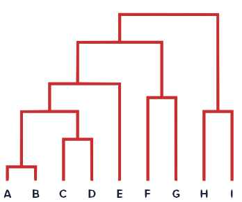
To closely examine amplicon sequencing data and to extract the unique 16S sequence variants from these, there is an incredibly useful package in R called DADA2. You have been provided with a small R script (reads2counts.r) which uses this package to count the abundance of each unique sequence in each sample. Based on these abundances, the script can compare samples to each other and can construct a distance tree (also known as a dendrogram):
The script takes the preprocessed forward & reverse reads (in no specific order) as input arguments on the command line.
Write and incorporate a process that executes this Rscript and outputs the counts_matrix.csv and dendrogram.png files.
The container that you use should have the R-package ‘DADA2’ installed.
You now have successfully written your own microbiomics pipeline!
Step 5: Rinse and repeat#
To see if all this effort in automatisation was really worth it, you should run your pipeline on another dataset to see if it works as well.
Run your pipeline on the sequencing data in the data2 directory.
If you have time left#
There are a few things left that you can implement in your pipeline so others can more easily work with it as well.
Use directives to output data from different processes to separate directories.
Make a cool header that displays every time you run your pipeline using the
log.infocommand.Add an onComplete printout to your pipeline that tells the user where they can find the output files.
Speed up the slow processes in your pipeline by allocating more cpus and memory to them.
Have nextflow create a report when you run the pipeline to see some cool stats.